Build Network#
Rule build_base_network#
Relevant Settings
interconnect:
offshore_shape:
aggregation_zones:
countries:
Inputs
data/breakthrough_network/base_grid/{interconnect}/bus.csvdata/breakthrough_network/base_grid/{interconnect}/branch.csvdata/breakthrough_network/base_grid/{interconnect}/dcline.csvdata/breakthrough_network/base_grid/{interconnect}/bus2sub.csvdata/breakthrough_network/base_grid/{interconnect}/sub.csvresources/country_shapes.geojson: confer Rule build_shapesresources/offshore_shapes.geojson: confer Rule build_shapesresources/{interconnect}/state_boundaries.geojson: confer Rule build_shapes
Outputs
networks/base.nc:data/breakthrough_network/base_grid/{interconnect}/bus2sub.csvdata/breakthrough_network/base_grid/{interconnect}/sub.csvresources/{interconnect}/elec_base_network.nc
Description
- Reads in Breakthrough Energy/TAMU transmission dataset, and converts it into PyPSA compatible components. A base netowork file (*.nc) is written out. Included in this network are:
Geolocated buses
Geoloactated AC and DC transmission lines + links
Transformers
Rule build_shapes#
Description
The build_shapes rule builds the GIS shape files for the balancing authorities and offshore regions. The regions are only built for the {interconnect} wildcard. Because balancing authorities often overlap- we modify the GIS dataset developed by [Breakthrough Energy Sciences](https://breakthrough-energy.github.io/docs/).
Relevant Settings
interconnect:
Inputs
breakthrough_network/base_grid/zone.csv: confer Rule build_base_networkrepo_data/BA_shapes_new/Modified_BE_BA_Shapes.shp: confer Rule build_base_networkrepo_data/BOEM_CA_OSW_GIS/CA_OSW_BOEM_CallAreas.shp: confer Rule build_base_network
Outputs
resources/country_shapes.geojson:# .. image:: ../img/regions_onshore.png # :scale: 33 %
resources/onshore_shapes.geojson:# .. image:: ../img/regions_offshore.png # :scale: 33 %
resources/offshore_shapes.geojson:# .. image:: ../img/regions_offshore.png # :scale: 33 %
resources/state_boundaries.geojson:# .. image:: ../img/regions_offshore.png # :scale: 33 %
Rule build_bus_regions#
Description
Creates Voronoi shapes for each bus representing both onshore and offshore regions.
Relevant Settings
interconnect:
aggregation_zones:
Inputs
resources/country_shapes.geojson: confer Rule build_shapesresources/offshore_shapes.geojson: confer Rule build_shapesnetworks/base.nc: confer Rule build_base_network
Outputs
resources/regions_onshore.geojsonresources/regions_offshore.geojson
Rule build_demand#
Builds the demand data for the PyPSA network.
Relevant Settings
network_configuration:

snapshots:
    start:
    end:
    inclusive:

scenario:
interconnect:
planning_horizons:
Inputs
base_network:
eia: (GridEmissions data file)
efs: (NREL EFS Load Forecasts)
Outputs
demand: Path to the demand CSV file.
Rule build_fuel_prices#
Description
Build_fuel_prices.py is a script that prepares data for dynamic fuel prices to be used in the add_electricity module. Data is input from retrieve_caiso_data and retrieve_eia_data to create a combined dataframe with all dynamic fuel prices available. The prices are modified to be on an hourly basis to match the network snapshots, and converted to $/MWh_thermal. The output is a CSV file containing the hourly fuel prices for each Balancing Authority and State.
Relevant Settings
fuel_year:
snapshots:
Inputs
‘’data/caiso_ng_prices.csv’’: A CSV file containing the daily average fuel prices for each Balancing Authority in the WEIM.
‘’data/eia_ng_prices.csv’’: A CSV file containing the monthly average fuel prices for each State.
Outputs
‘’data/ng_fuel_prices.csv’’: A CSV file containing the hourly fuel prices for each Balancing Authority and State.
Rule build_cutout#
Create cutouts with atlite.
For this rule to work you must have
installed the Copernicus Climate Data Store
cdsapipackage (install with `pip`) andregistered and setup your CDS API key as described on their website.
See also
For details on the weather data read the atlite documentation. If you need help specifically for creating cutouts the corresponding section in the atlite documentation should be helpful.
Relevant Settings
atlite:
    nprocesses:
    cutouts:
        {cutout}:
See also
Documentation of the configuration file config/config.yaml at
atlite
Inputs
None
Outputs
cutouts/{cutout}: weather data from the ERA5 reanalysis weather dataset satellite-based historic weather data with the following structure:
Description
Using the ERA5 cutout, the following parameters are accessible:
Field
Dimensions
Unit
Description
height
y, x
m
Surface elevation above sea level
wnd100m
time, y, x
ms**-1
Wind speeds at 100 meters (regardless of direction)
wnd_azimuth
time, y, x
ms**-1
100 metre U wind component
roughness
y, x
m
Forecast surface roughness (roughness length)
influx_toa
time, y, x
Wm**-2
Top of Earth’s atmosphere TOA incident solar radiation
influx_direct
time, y, x
Wm**-2
Total sky direct solar radiation at surface
influx_diffuse
time, y, x
Wm**-2
Diffuse solar radiation at surface. Surface solar radiation downwards minus direct solar radiation.
solar_altitude
time, y, x
rad
solar_azimuth
time, y, x
rad
temperature
time, y, x
K
Air temperature 2 meters above the surface.
soil temperature
time, y, x
K
Soil temperature between 1 meters and 3 meters depth (layer 4).
influx_toa
time, y, x
Wm**-2
Top of Earth’s atmosphere TOA incident solar radiation
influx_direct
time, y, x
Wm**-2
Total sky direct solar radiation at surface
runoff
time, y, x
m
Runoff (volume per area)
albedo
time, y, x
–
Albedo measure of diffuse reflection of solar radiation. Calculated from relation between surface solar radiation downwards (Jm**-2) and surface net solar radiation (Jm**-2). Takes values between 0 and 1.
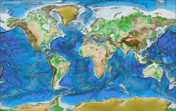
The USA Interconnect weather data is shown below:

Rule build_renewable_profiles#
Calculates for each network node the (i) installable capacity (based on land- use), (ii) the available generation time series (based on weather data), and (iii) the average distance from the node for onshore wind, AC-connected offshore wind, DC-connected offshore wind and solar PV generators. In addition for offshore wind it calculates the fraction of the grid connection which is under water.
Note
Hydroelectric profiles are built in script build_hydro_profiles.
Relevant settings
snapshots:

atlite:
    nprocesses:

renewable:
    {technology}:
        cutout:
        corine:
        grid_codes:
        distance:
        natura:
        min_depth:
        max_depth:
        max_shore_distance:
        min_shore_distance:
        capacity_per_sqkm:
        correction_factor:
        potential:
        min_p_max_pu:
        clip_p_max_pu:
        resource:
Inputs
data/bundle/corine/g250_clc06_V18_5.tif: CORINE Land Cover (CLC) inventory on 44 classes of land use (e.g. forests, arable land, industrial, urban areas).# .. image:: img/corine.png # :scale: 33 %
data/bundle/GEBCO_2014_2D.nc: A bathymetric data set with a global terrain model for ocean and land at 15 arc-second intervals by the General Bathymetric Chart of the Oceans (GEBCO).# .. image:: img/gebco_2019_grid_image.jpg # :scale: 50 %
Source: GEBCO
resources/natura.tiff: confer Rule retrieve_zenodo_databundlesresources/offshore_shapes.geojson: confer Rule build_shapesresources/regions_onshore.geojson: (if not offshore wind), confer Rule build_bus_regionsresources/regions_offshore.geojson: (if offshore wind), Rule build_bus_regions"cutouts/" + params["renewable"][{technology}]['cutout']: Rule build_cutoutnetworks/base.nc: Rule build_base_network
Outputs
resources/profile_{technology}.nc with the following structure
Field
Dimensions
Description
profile
bus, time
the per unit hourly availability factors for each node
weight
bus
sum of the layout weighting for each node
p_nom_max
bus
maximal installable capacity at the node (in MW)
potential
y, x
layout of generator units at cutout grid cells inside the Voronoi cell (maximal installable capacity at each grid cell multiplied by capacity factor)
average_distance
bus
average distance of units in the Voronoi cell to the grid node (in km)
underwater_fraction
bus
fraction of the average connection distance which is under water (only for offshore)
profile
# .. image:: img/profile_ts.png # :scale: 33 % # :align: center
p_nom_max
# .. image:: img/p_nom_max_hist.png # :scale: 33 % # :align: center
potential
# .. image:: img/potential_heatmap.png # :scale: 33 % # :align: center
average_distance
# .. image:: img/distance_hist.png # :scale: 33 % # :align: center
underwater_fraction
# .. image:: img/underwater_hist.png # :scale: 33 % # :align: center
Description#
This script functions at two main spatial resolutions: the resolution of the network nodes and their Voronoi cells, and the resolution of the cutout grid cells for the weather data. Typically the weather data grid is finer than the network nodes, so we have to work out the distribution of generators across the grid cells within each Voronoi cell. This is done by taking account of a combination of the available land at each grid cell and the capacity factor there.
First the script computes how much of the technology can be installed at each cutout grid cell and each node using the GLAES library. This uses the CORINE land use data, Natura2000 nature reserves and GEBCO bathymetry data.
To compute the layout of generators in each node’s Voronoi cell, the installable potential in each grid cell is multiplied with the capacity factor at each grid cell. This is done since we assume more generators are installed at cells with a higher capacity factor.
This layout is then used to compute the generation availability time series from the weather data cutout from atlite.
Two methods are available to compute the maximal installable potential for the node (p_nom_max): simple and conservative:
simple adds up the installable potentials of the individual grid cells. If the model comes close to this limit, then the time series may slightly overestimate production since it is assumed the geographical distribution is proportional to capacity factor.
conservative assertains the nodal limit by increasing capacities proportional to the layout until the limit of an individual grid cell is reached.
Rule add_electricity#
Description
This module integrates data produced by build_renewable_profiles, build_demand, build_cost_data, build_fuel_prices, and build_base_network to create a network model that includes generators, demand, and costs. The module attaches generators, storage units, and loads to the network created by build_base_network. Each generator is assigned regional capital costs, and regional and daily or monthly marginal costs.
Extendable generators are assigned a maximum capacity based on land-use constraints defined in build_renewable_profiles.
Relevant Settings
network_configuration:

snapshots:
    start:
    end:
    inclusive:

electricity:
See also
Documentation of the configuration file config/config.yaml at costs, electricity, renewable, lines
Inputs
resources/costs.csv: The database of cost assumptions for all included technologies for specific years from various sources; e.g. discount rate, lifetime, investment (CAPEX), fixed operation and maintenance (FOM), variable operation and maintenance (VOM), fuel costs, efficiency, carbon-dioxide intensity.resources/demand.csvHourly per-country load profiles.resources/regions_onshore.geojson: confer Rule build_bus_regionsresources/profile_{}.nc: all technologies inconfig["renewables"].keys(), confer Rule build_renewable_profiles.networks/elec_base_network.nc: confer Rule build_base_networkresources/ng_fuel_prices.csv: Natural gas fuel prices by state and BA.
Outputs
networks/elec_base_network_l_pp.nc